Transport
of segments
In the Euclidean
Geometry, we know that
there are some applications that preserve
the distances and the angles. These applications, called isometries,
are the rotations and the translations. The
isometries bring lines to lines and segments to
segments of the same length. To apply a translation we have to know the
direction and the distance and to apply a rotation we have to know the
angle.
In the
Hyperbolic Geometry we have also isometries. In the half-plane model,
the isometries are composition of inversions with respect to
circumferences with center in the boundary line. To fix an
isometry it is
necessary to fix a point in the boundary line (which
will be the center of the circumference of inversion) and a
distance (which will be the radius of the circumference of
inversion).
From the isometries we will be able to transport the objects of the
Hyperbolic Geometry.
This sketch allows us to transport a segment to another position. We
have to fix the beginning of the transported segment and the direction,
that is, it is necessary to fix a point and a ray. To make the
transport we will use two isometries.
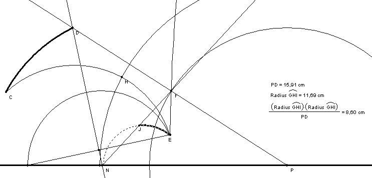
To make the transport of a segment CD
to the ray with end E we have
followed these steps:
- Plot the hyperbolic segment CE.
- Plot the
hyperbolic perpendicular
bisector of
the hyperbolic segment CE.
We consider as
inversion circumference the
circumference that describes this perpendicular bisector. We apply the
inversion to the points C and
D. C transforms into E since, by construction,
the inversion circumference passes through the midpoint of the
segment CE.
- Plot
the Euclidean line that joins the points C and E.
- Consider
the intersection point between the former line and the boundary line.
This point, P, is the center
of the inversion
circumference.
- Measure
the radius, r, of the
circumference of inversion. We can make it selecting the
circumference and the tool "Measure/Radius".
- Calculate
the distance between the point D
and its image by the
inversion that we are considering. We can find this distance
from the inversion's definition, that is, from
the formula: PD = r·r/PC.
- Plot the
Euclidean circumference of center P and radius the former
result.
- Plot the
Euclidean line that joins the
points P and D.
- Consider
the intersection between the circumference in step (7) with the line in
step (8). This point, F, is
the
image of D by the
inversion.
- Plot the
hyperbolic bisector of the angle that has for vertex the
point E and for side EF and the given ray.
We
consider as another inversion circumference, the
circumference that determine the bisector. We apply the
inversion in the points E and F. The point E is
fixed for the inversion to belong to the
circumference of inversion. As the inversions preserve the angles, the
ray EF transforms with the
given ray. Thus, the image of F
by this inversion
will determine the end of the transported segment. From now, we cannot
follow a method analogous to that of the steps (3)-(9) because we know
the image of a fixed point, so, we
cannot plot the line for the point and its
image.
- Plot the segment that joins the
point E to the intersection
point of the bisector with the boundary line.
- Consider
the Euclidean midpoint of the former segment.
- Plot the
perpendicular line to the segment that goes through the midpoint.
- Consider
the intersection point of the former line with the boundary
line. This point is the center of the circumference of
inversion since it has been constructed from the perpendicular bisector
of a segment that joins two of the points of the
circumference.
- Plot the
Euclidean line that joins the former point with F.
- Consider
the intersection, J, of this
line with the given ray. This is the image of F and the
end of the segment that we searched.
- Plot the hyperbolic segment
that has endpoints in E and J.
This is the transported segment of the segment CD.
List of tools
Hyperbolic
geometry